Distill What You Want: A Unified View of On-Policy Distillation

English · 中文版

This is my first attempt at writing a full technical post on my personal website, so there are surely rough edges and places where the reasoning or exposition could be improved. If you notice anything inaccurate or unclear, or see an idea worth discussing further, I would be very grateful for your corrections and feedback—and I appreciate your patience.

You may have heard of On-Policy Distillation (OPD): the student generates data along its own trajectories and learns by matching the teacher’s probability distribution (Agarwal et al., 2024).

When there is only one teacher, this description may seem sufficient. But once we introduce multiple teachers or try to combine different distillation objectives, things quickly become more complicated: what exactly are we combining, and what do we ultimately want the student to learn?

In this post, I introduce a perspective that I find especially intuitive: turn a complex distillation problem into a simple problem of vector composition and matching.

From this perspective, we can not only understand OPD more easily, but also answer a more interesting question with greater freedom: if we can choose, what exactly do we want to distill from a model?

Probability distributions are somewhat awkward objects. We can compare two distributions, but it is hard to ask intuitively: what does one distribution contain beyond another? Can what two models have learned be added together? Can a particular capability be subtracted from a model?

If these probability distributions could be represented as ordinary vectors, the problem would become much simpler. We could use subtraction to describe changes between models, addition to combine changes from different models, and even decompose a complex distillation target into several simple directions.

In other words, we could turn a problem in probability space into a linear algebra problem.

Fortunately, such a tool exists.

The central thread of this post: use CLR to map probability distributions into a vector space, construct the target we want in that space, and then choose an appropriate divergence to make the student match that target.

To simplify notation, this post considers a token-level categorical distribution conditioned on the current context and omits the explicit conditioning on that context. For softmax outputs, every component is strictly positive, so the domain requirements of the CLR transformation below are satisfied.

1. Centered Log-Ratio Transformation

1.1. Why We Need CLR

Before discussing distillation further, let us first solve a more fundamental problem: how can we turn a probability distribution into a vector on which addition and subtraction are genuinely meaningful?

This is not a new problem. In fields such as computational biology, microbiome analysis, and analytical chemistry, researchers have long worked with a special type of data called compositional data (Aitchison, 1982). For such data, what matters is often not the absolute magnitude of each component, but the relative proportions among components. A probability distribution is a canonical example of compositional data.

A classical tool for bringing this kind of data into the familiar world of linear algebra is the Centered Log-Ratio (CLR) transformation.

Its central idea can be summarized in one sentence: turn ratios into coordinates, thereby turning a probability distribution into a vector that supports linear operations.

For a categorical distribution

\[p=(p_1,p_2,ldots,p_K), \qquad \sum_{i=1}^{K}p_i=1,\quad p_i>0,\]

its CLR transformation is defined as

\[C(p)_i = \log p_i- \frac{1}{K}\sum_{j=1}^{K}\log p_j.\]

Intuitively, CLR does not directly care about how large a particular $p_i$ is. Instead, it describes how large that component is relative to the other components of the distribution. This relative structure is exactly what later allows us to discuss directions, differences, and compositions between models.

1.2. Key Properties of CLR

CLR is useful for understanding distillation because it preserves the relative relationships that matter in a probability distribution while embedding the distribution in a space that supports linear operations.

1. The Components of a CLR Vector Always Sum to Zero

\[\sum_{i=1}^{K}C(p)_i=0.\]

Thus, although $C(p)$ has $K$ components, it has only $K-1$ degrees of freedom—exactly the same number as a categorical distribution over $K$ classes.

2. CLR Exactly Preserves Ratios Between Probabilities

\[C(p)_i-C(p)_j = \log\frac{p_i}{p_j}.\]

The difference between two coordinates in CLR space is precisely the log-ratio between the corresponding classes in the original probability distribution.

From this viewpoint, CLR does not discard the information that matters in a probability distribution. It simply expresses that information in coordinates that are more convenient for linear operations.

3. CLR Is Invariant to Global Scaling

For any $c>0$,

\[C(cp)=C(p).\]

This is because CLR cares only about relative proportions, not about a common scale applied to all components.

4. For Softmax Logits, CLR Is Just the Logits with Their Mean Removed

Suppose

\[p=\operatorname{softmax}(z).\]

Then

\[C(p)_i = z_i- \frac{1}{K}\sum_{j=1}^{K}z_j.\]

In other words, CLR simply subtracts the mean logit from every logit.

This matters especially for distillation because softmax itself is invariant to a global translation:

\[\operatorname{softmax}(z+c\mathbf{1}) = \operatorname{softmax}(z).\]

CLR can therefore be understood as a canonical coordinate system for logits: it preserves all relative structure that affects the probability distribution while removing the global offset that softmax ignores.

1.3. The Inverse Transformation

CLR not only maps a probability distribution into a vector space; the mapping is also invertible.

Given a CLR vector

\[z=C(p),\]

we can recover the original probability distribution through softmax:

\[p_i = \frac{e^{z_i}}{\sum_{j=1}^{K}e^{z_j}} = \operatorname{softmax}(z)_i.\]

For categorical distributions whose components are all strictly positive, CLR therefore establishes a one-to-one correspondence between the interior of the probability simplex and the following zero-sum vector space:

\[\left\{ z\in\mathbb{R}^K \;\middle|\; \sum_{i=1}^{K}z_i=0 \right\}.\]

That is, the CLR transformation loses no information from the probability distribution: every probability distribution corresponds to a unique CLR vector, and every zero-sum CLR vector can be mapped back to a unique probability distribution through softmax.

We can therefore map probability distributions into CLR space, operate on them with familiar vector addition, subtraction, and linear algebra, and then return to probability space through softmax.

1.4. Bonus: Aitchison Geometry

If we take one more step, we find that CLR is not merely an accidentally convenient transformation.

Probability distributions are a special kind of compositional data. For this kind of data, the absolute magnitudes of individual components are less meaningful than their ratios. Ordinary addition and distance in Euclidean space are therefore not the most natural operations.

Aitchison geometry is a geometry designed specifically for data whose relative proportions are what matter (Aitchison, 1986).

In Aitchison geometry, “adding” two compositions does not mean adding their components elementwise. Instead, we multiply corresponding components and then renormalize. For two probability distributions $p$ and $q$, this operation can be written as

\[p\oplus q = \mathcal{C}(p_1q_1,\ldots,p_Kq_K),\]

where $\mathcal{C}$ renormalizes the components so that they sum to one.

Similarly, “scalar multiplication” of a distribution corresponds to raising each component to a power and then renormalizing:

\[\alpha\odot p = \mathcal{C}(p_1^\alpha,\ldots,p_K^\alpha).\]

These operations may look unfamiliar, but this is where CLR becomes elegant:

\[C(p\oplus q)=C(p)+C(q),\]

and

\[C(\alpha\odot p)=\alpha C(p).\]

In other words, addition and scalar multiplication in Aitchison geometry become ordinary vector addition and scalar multiplication after the CLR transformation.

CLR does more than merely turn a probability distribution into a vector. More precisely, it turns the latent linear structure of the probability simplex into the familiar linear structure of Euclidean space.

This is why we can safely use the language of vectors to discuss policy composition, differences, and directions in the sections that follow.

2. A Vector Interpretation of OPD

With CLR in hand, we can reconsider OPD.

OPD is often written directly as a KL divergence or another loss, followed by a discussion of whether to use Forward KL, Reverse KL, or some other similarity measure.

But this formulation conflates two separate questions:

1. Which distribution do we want OPD to learn?
2. How should we measure the difference between the student distribution and the target distribution?

Under the perspective developed here, we separate these questions explicitly.

The first is Target Distribution Construction. We map the teacher, student, reference model, and other relevant distributions into CLR space; use vector addition, subtraction, scaling, and composition to construct the target vector that we actually want the student to learn; and finally apply the inverse transformation to obtain the corresponding target distribution.

The second is Similarity Measurement. Once the target distribution has been determined, we choose an appropriate way to measure the difference between the student and target distributions, such as Forward KL, Reverse KL, or Jensen-Shannon Divergence.

2.1. Target Distribution Construction: Define What We Want to Learn with Vector Operations

From this perspective, the first step of OPD is not to write down a loss. It is to answer a more fundamental question:

Which distribution do we actually want the student to learn?

With CLR, this becomes a simple three-step process:

1. Map the relevant model distributions into CLR space.
2. Construct a target vector through vector operations in CLR space.
3. Map the target vector back to a target distribution through softmax.

That is, Target Distribution Construction is fundamentally

\[p_1,p_2,\ldots,p_n \xrightarrow{\text{CLR}} c_1,c_2,\ldots,c_n \xrightarrow{\text{Vector Operations}} c_{\text{target}} \xrightarrow{\text{Softmax}} p_{\text{target}}.\]

Let us examine several common examples.

Example 1: Traditional OPD

Classical knowledge distillation transfers knowledge by making a student match a teacher’s soft outputs (Hinton et al., 2015). Its on-policy variant performs this matching on sequences generated by the student itself (Agarwal et al., 2024).

Traditional OPD has one teacher $T$ and one student $S$. In this case, the target distribution is simple: it is the teacher distribution itself.

Let

\[c_S=C(p_S), \qquad c_T=C(p_T).\]

The most direct target construction is

\[c_{\text{target}}=c_T.\]

From a vector perspective, this can also be written as

\[c_{\text{target}} = c_S+(c_T-c_S).\]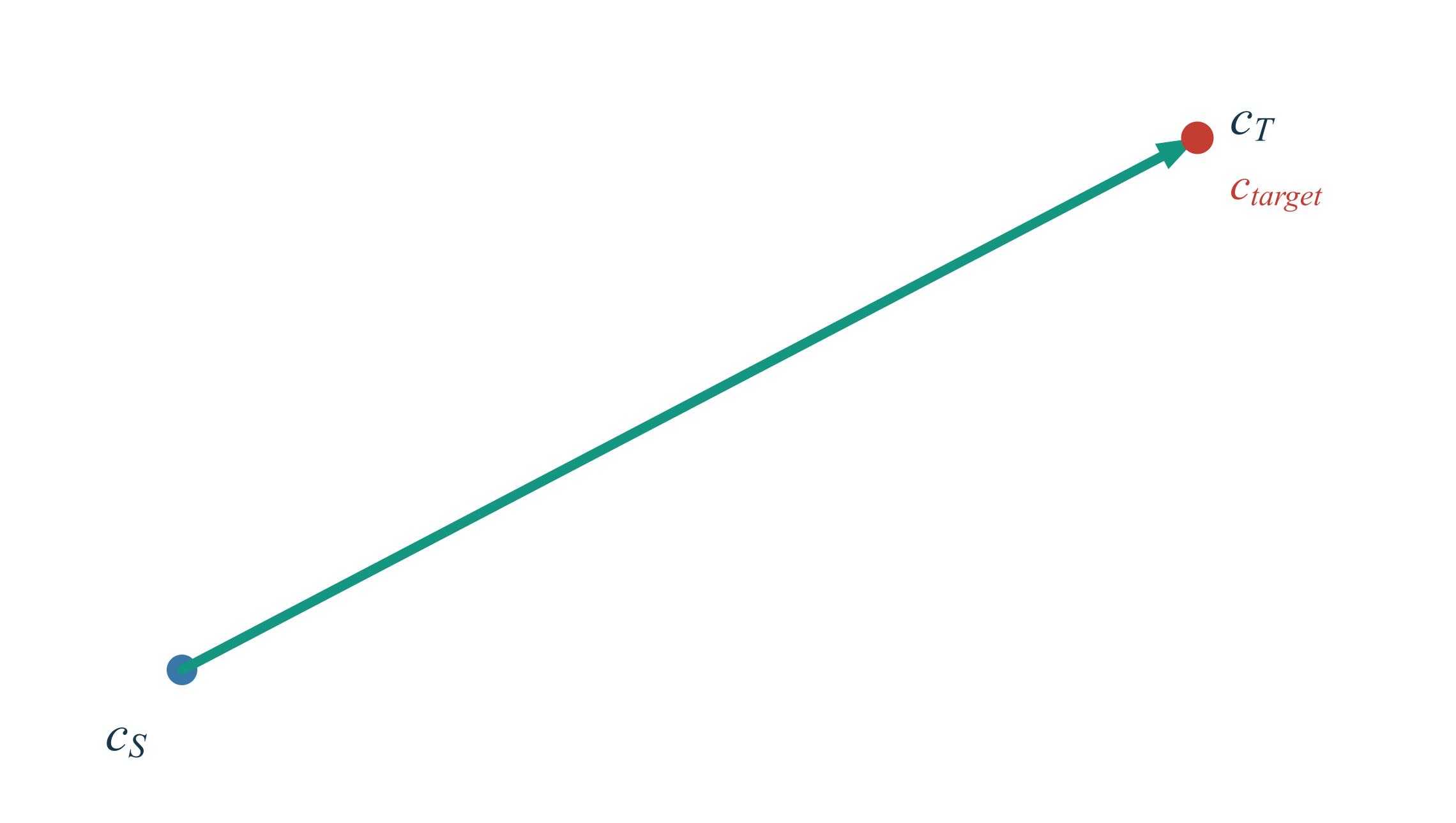

We start at the student’s current position $c_S$ and move along the direction

\[c_T-c_S\]

until we reach the teacher’s position.

Applying the inverse CLR transformation gives

\[p_{\text{target}} = \operatorname{softmax}(c_{\text{target}}) = \operatorname{softmax}(c_T) = p_T.\]

Traditional OPD therefore has a very simple interpretation under this view:

Move the student to the teacher’s position.

Example 2: Weak-to-Strong Distillation

Now consider a more interesting setting: a weak reference model $W$, a reinforced weak teacher $T$, and a stronger student $S$ that we want to train.

This is the weak-to-strong transfer setting studied by Direct On-Policy Distillation (Direct-OPD). Instead of imitating the weak teacher’s final distribution, Direct-OPD transfers the policy shift from the weak model before training to the weak model after training (Feng et al., 2026). In the paper’s notation, $W$ is the pre-RL teacher reference and $T$ is the post-RL teacher. Here, we describe the same direction of change directly in CLR space.

If our goal is merely to copy the teacher, we can still set

\[c_{\text{target}}=c_T.\]

But from the vector perspective, we can instead distill the improvement direction of the post-RL teacher relative to the pre-RL reference:

\[\Delta_{W\rightarrow T} = c_T-c_W.\]

We then translate this improvement vector to the student’s current position:

\[c_{\text{target}} = c_S+\alpha(c_T-c_W),\]

where $\alpha>0$ controls the strength with which we apply the improvement.

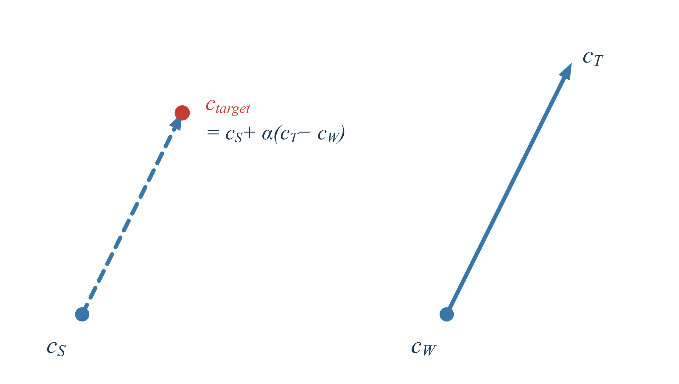
The corresponding target distribution is

\[p_{\text{target}} = \operatorname{softmax} \left( c_S+\alpha(c_T-c_W) \right).\]

We can also express this target directly in probability space. By the definition of CLR,

\[c_i(p) = \log p_i- \frac{1}{K}\sum_j\log p_j,\]

so

\[c_{\text{target},i} = \log p_{S,i} +\alpha\log p_{T,i} -\alpha\log p_{W,i} +\text{constant}.\]

After softmax, the constant independent of $i$ cancels, giving

\[p_{\text{target},i} \propto p_{S,i} \left( \frac{p_{T,i}}{p_{W,i}} \right)^\alpha.\]

After normalization,

\[p_{\text{target},i} = \frac{ p_{S,i} \left( \frac{p_{T,i}}{p_{W,i}} \right)^\alpha }{ \sum_j p_{S,j} \left( \frac{p_{T,j}}{p_{W,j}} \right)^\alpha }.\]

Under this view, we do not distill the weak teacher itself. We distill the training-induced change that it exhibits relative to its own reference:

Instead of copying the weak teacher, transfer the weak teacher’s improvement over its own reference to the stronger student.

This has the same form as the idealized optimal policy in Direct-OPD. That paper writes the exponent as the inverse of a KL coefficient, whereas this post uses $\alpha$ directly as the transfer strength of the policy shift. If implemented as explicit target matching, the target changes with the current student, so one must specify whether to stop gradients through the target branch. Direct-OPD itself instead treats the teacher shift as an implicit reward and anchors the student to its initialization with a KL term.

Example 3: Multi-Teacher On-Policy Distillation

Finally, consider multiple teachers. Recent frontier-model technical reports use Multi-Teacher On-Policy Distillation (MOPD) as a central post-training method for integrating the capabilities of domain specialists. MiMo-V2-Flash independently trains specialized teachers for mathematics, reasoning, safety, agents, and other domains, then applies token-level KL supervision from the appropriate domain teacher to student rollouts (Xiaomi LLM-Core Team, 2026). DeepSeek-V4 uses a similar specialist-then-distill pipeline: it first trains multiple domain experts and then merges the capabilities of more than ten teachers into a unified model through weighted reverse KL on student-generated trajectories (DeepSeek-AI, 2026).

From the CLR perspective, whether a system uses hard routing to select a teacher by domain or soft weighting to compute multiple teacher losses simultaneously, the core problem is how to integrate supervision from

\[T_1,T_2,\ldots,T_M.\]

One natural way to combine multiple teachers in CLR space is to take a linear combination of their vectors:

\[c_{\text{target}} = \sum_{m=1}^{M}\alpha_m c_{T_m},\]

where we typically choose

\[\alpha_m\geq 0, \qquad \sum_{m=1}^{M}\alpha_m=1.\]

The weights $\alpha_m$ may also depend on the current context $x$. A one-hot $\alpha_m(x)$ corresponds to the domain-routed teacher selection described by MiMo-V2-Flash. Multiple nonzero weights correspond to a more general weighted multi-teacher objective, such as the weighted reverse-KL objective reported for DeepSeek-V4.

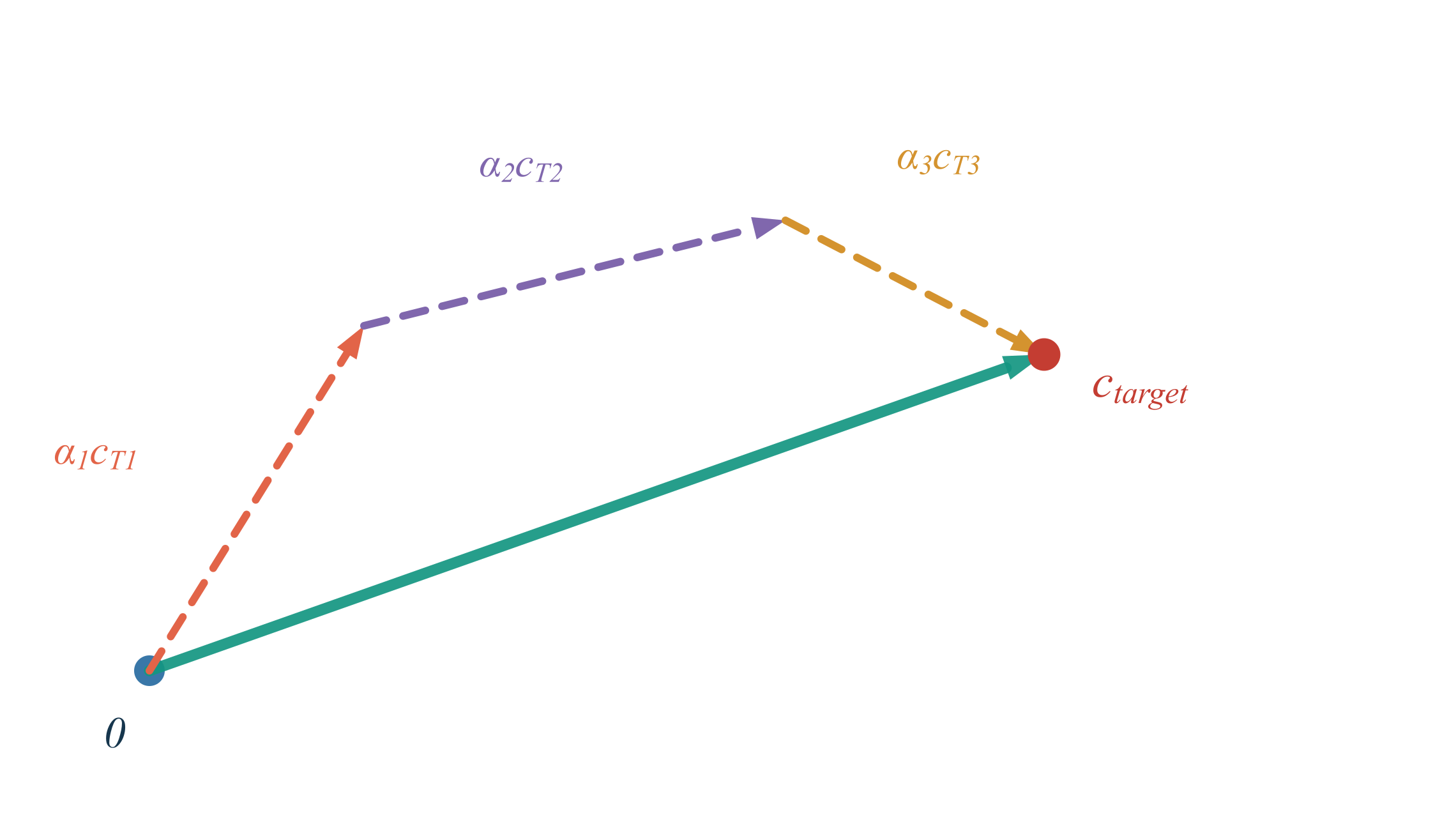
The corresponding target distribution is

\[p_{\text{target}} = \operatorname{softmax} \left( \sum_{m=1}^{M}\alpha_m c_{T_m} \right).\]

Using the definition of CLR,

\[\sum_{m=1}^{M}\alpha_m c_{T_m,i} = \sum_{m=1}^{M}\alpha_m\log p_{T_m,i} +\text{constant},\]

and therefore

\[p_{\text{target},i} \propto \exp \left( \sum_{m=1}^{M}\alpha_m\log p_{T_m,i} \right) = \prod_{m=1}^{M}p_{T_m,i}^{\alpha_m}.\]

After normalization,

\[p_{\text{target},i} = \frac{ \prod_{m=1}^{M}p_{T_m,i}^{\alpha_m} }{ \sum_j\prod_{m=1}^{M}p_{T_m,j}^{\alpha_m} }.\]

Thus, a convex combination in CLR space corresponds to a normalized weighted geometric mean in probability space. Allowing negative weights or weights that do not sum to one gives a more general linear combination, but no longer a convex combination of teachers in the usual sense.

More generally, we do not have to combine the teachers themselves. We can combine the improvement vectors provided by multiple teachers.

For example, relative to a reference model $R$,

\[c_{\text{target}} = c_S+ \sum_{m=1}^{M}\alpha_m(c_{T_m}-c_R).\]

The corresponding target distribution is

\[p_{\text{target},i} \propto p_{S,i} \prod_{m=1}^{M} \left( \frac{p_{T_m,i}}{p_{R,i}} \right)^{\alpha_m}.\]

Here, what we combine is no longer the absolute distributions of multiple teachers, but their respective directions of change relative to the reference model.

Multi-teacher distillation is fundamentally a decision about which vectors to combine in CLR space.

2.2. Constructing the Loss with a Similarity Measure

After constructing the target distribution, the next question is: how should we make the student approach that target?

We first need to distinguish between on-policy and off-policy training.

The definition of on-policy is direct: the samples used for training are generated by the current student model itself.

If the student policy is $\pi_S$, the training trajectory is sampled as

\[\tau\sim\pi_S.\]

The student generates according to its current policy. We then construct target distributions and compute the corresponding distillation loss on the contexts that the student itself visits.

By contrast, in off-policy training, the samples are not generated by the current student. They may come from a teacher, another policy, or a fixed dataset collected in advance.

For example,

\[\tau\sim\pi_T,\]

or, more generally,

\[\tau\sim\mathcal{D}.\]

On-policy and off-policy therefore describe where the training contexts or trajectories come from, not how we compare two token-level probability distributions. These are independent design dimensions.

Once the training samples have been determined, we choose a similarity measure—such as Forward KL, Reverse KL (Kullback and Leibler, 1951), or Jensen-Shannon Divergence (JSD; Lin, 1991)—to measure the difference between the student and target distributions.

Forward KL

\[D_{\mathrm{KL}} \left( p_{\text{target}}\Vert p_S \right) = \sum_i p_{\text{target},i} \log\frac{p_{\text{target},i}}{p_{S,i}}.\]

Equivalently, in expectation form,

\[D_{\mathrm{KL}} \left( p_{\text{target}}\Vert p_S \right) = \mathbb{E}_{x\sim p_{\text{target}}} \left[ \log\frac{p_{\text{target}}(x)}{p_S(x)} \right].\]

Forward KL therefore takes its expectation under the target distribution.

Reverse KL

\[D_{\mathrm{KL}} \left( p_S\Vert p_{\text{target}} \right) = \sum_i p_{S,i} \log\frac{p_{S,i}}{p_{\text{target},i}}.\]

Equivalently,

\[D_{\mathrm{KL}} \left( p_S\Vert p_{\text{target}} \right) = \mathbb{E}_{x\sim p_S} \left[ \log\frac{p_S(x)}{p_{\text{target}}(x)} \right].\]

Here the expectation is taken under the student distribution.

Jensen-Shannon Divergence (JSD)

First define the mixture distribution

\[m = \frac{1}{2} \left( p_S+p_{\text{target}} \right).\]

JSD is then defined as

\[D_{\mathrm{JS}} \left( p_S,p_{\text{target}} \right) = \frac{1}{2} D_{\mathrm{KL}} \left( p_S\Vert m \right) + \frac{1}{2} D_{\mathrm{KL}} \left( p_{\text{target}}\Vert m \right).\]

Expanded as sums,

\[D_{\mathrm{JS}} \left( p_S,p_{\text{target}} \right) = \frac{1}{2} \sum_i p_{S,i} \log\frac{p_{S,i}}{m_i} + \frac{1}{2} \sum_i p_{\text{target},i} \log\frac{p_{\text{target},i}}{m_i}.\]

It can also be written in expectation form:

\[D_{\mathrm{JS}} \left( p_S,p_{\text{target}} \right) = \frac{1}{2} \mathbb{E}_{x\sim p_S} \left[ \log\frac{p_S(x)}{m(x)} \right] + \frac{1}{2} \mathbb{E}_{x\sim p_{\text{target}}} \left[ \log\frac{p_{\text{target}}(x)}{m(x)} \right],\]

where

\[m(x) = \frac{1}{2} \left( p_S(x)+p_{\text{target}}(x) \right).\]

Unlike Forward KL and Reverse KL, JSD measures the difference between both the student and target distributions and their mixture $m$. It is therefore symmetric:

\[D_{\mathrm{JS}} \left( p_S,p_{\text{target}} \right) = D_{\mathrm{JS}} \left( p_{\text{target}},p_S \right).\]

2.3. Equivalence Between CLR Target Construction and Traditional Distillation Objectives

So far, we have constructed a target distribution in CLR space and then matched that target. A natural question is:

How does this “construct the target first” formulation differ from writing a conventional distillation objective directly?

The answer is: under suitable conditions, the two formulations are equivalent. We can see this by using Reverse KL as the objective.

Start with the simplest, single-teacher case. Since

\[c_{\text{target}}=c_T,\]

we have

\[p_{\text{target}}=p_T,\]

and therefore

\[D_{\mathrm{KL}}(p_S\Vert p_{\text{target}}) = D_{\mathrm{KL}}(p_S\Vert p_T).\]

The multi-teacher case is more interesting.

Suppose we construct

\[c_{\text{target}} = \sum_{m=1}^{M}\alpha_m c_{T_m}, \qquad \sum_{m=1}^{M}\alpha_m=1\]

in CLR space. The corresponding target distribution is

\[p_{\text{target},i} = \frac{ \prod_{m=1}^{M}p_{T_m,i}^{\alpha_m} }{Z},\]

where

\[Z = \sum_j\prod_{m=1}^{M}p_{T_m,j}^{\alpha_m}.\]

Now apply Reverse KL to this target:

\[D_{\mathrm{KL}} \left( p_S\Vert p_{\text{target}} \right) = \mathbb{E}_{x\sim p_S} \left[ \log p_S(x)-\log p_{\text{target}}(x) \right].\]

Substituting the target distribution,

\[D_{\mathrm{KL}} \left( p_S\Vert p_{\text{target}} \right) = \mathbb{E}_{x\sim p_S} \left[ \log p_S(x) -\sum_{m=1}^{M}\alpha_m\log p_{T_m}(x) +\log Z \right].\]

Because $\sum_m\alpha_m=1$, this can be rearranged as

\[D_{\mathrm{KL}} \left( p_S\Vert p_{\text{target}} \right) = \sum_{m=1}^{M} \alpha_m D_{\mathrm{KL}} \left( p_S\Vert p_{T_m} \right) +\log Z.\]

For fixed context, teachers, and weights $\alpha_m$, the term $\log Z$ is independent of the current token-level student distribution. Therefore, when optimizing the student under these conditions,

\[\boxed{ D_{\mathrm{KL}} \left( p_S\Vert p_{\text{target}} \right) \equiv \sum_{m=1}^{M} \alpha_m D_{\mathrm{KL}} \left( p_S\Vert p_{T_m} \right) }\]

where $\equiv$ means that the two expressions differ only by a constant independent of the current token-level student distribution, and thus have the same local optimization objective and gradient.

In other words, the traditional multi-teacher Reverse-KL objective

\[\sum_m \alpha_m D_{\mathrm{KL}} \left( p_S\Vert p_{T_m} \right)\]

implicitly defines a very specific target distribution:

\[p_{\text{target},i} \propto \prod_m p_{T_m,i}^{\alpha_m}.\]

CLR makes explicit the target distribution that was previously hidden inside the objective.

The equivalence above concerns a token-level loss at a fixed context. If we further differentiate through the distribution of on-policy trajectories, the contexts themselves vary with the student policy, and the exact treatment of sampling and gradient estimation must also be specified.

3. What CLR Reveals About Distillation

So far, we have primarily treated CLR as a tool for target construction: vector operations let us construct the target distribution we want.

CLR has another advantage: it makes many training phenomena that are hidden in probability space visually and algebraically transparent.

Once every policy is represented as a vector, we can directly examine the following properties of distillation signals:

• Components: which changes are the information increments we actually want to transfer to the student;
• Directions: where different teachers want to move the student;
• Angles: whether different teachers provide consistent supervision;
• Lengths: how much new learning signal a teacher still provides relative to the student;
• Resultants: how much effective signal remains after multiple distillation targets are combined.

We now consider three things the CLR view can reveal: how to construct desired information components, how to identify multi-teacher conflict, and how to monitor distillation progress.

3.1. Distill the Components You Want: Constructing Targets from Information Increments

Most targets discussed so far come from a complete teacher distribution. The more interesting implication of the CLR perspective is that we do not have to distill a model as a whole; we can distill a particular segment of change between models.

Suppose we have a pair of models $A_k^{-}$ and $A_k^{+}$, representing the model before and after the addition of the $k$-th training signal, respectively, with both models sharing the same token space. We define their CLR difference as

\[\Delta_k = C\left(p_{A_k^{+}}\right) - C\left(p_{A_k^{-}}\right).\]

If the only major change between the two models is that the latter learned the capability, preference, or behavior of interest, then $\Delta_k$ can be interpreted as the information increment contributed by that component.

For example:

• The difference between pre-RL and post-RL checkpoints can represent the policy shift introduced by RL. Direct-OPD treats precisely this kind of change as a transferable supervision signal (Feng et al., 2026).
• The difference before and after domain fine-tuning can approximate the knowledge increment introduced by that domain.
• The difference before and after preference tuning can approximate a particular preference or behavioral constraint.
• The difference between checkpoints from two training stages can describe what that stage changed.
• A distributional difference induced by two different inputs can represent the information difference between those inputs.

Once we obtain an information increment, we can translate it to the student’s current position:

\[c_{\text{target}} = c_S+\alpha_k\Delta_k.\]

The student does not need to copy the complete distribution of $A_k^{+}$. Starting from its own current position, it only needs to learn the segment of change extracted from the model pair.

If we want to transfer multiple components simultaneously, we can write

\[c_{\text{target}} = c_S+ \sum_{k=1}^{K}\alpha_k\Delta_k,\]

where each $\alpha_k$ controls the strength of its information component. A positive $\alpha_k$ adds or amplifies that direction, $\alpha_k=0$ ignores it, and a negative $\alpha_k$ attempts to suppress or reverse the change.

In probability space, this becomes

\[p_{\text{target},i} \propto p_{S,i} \prod_{k=1}^{K} \left( \frac{ p_{A_k^{+},i} }{ p_{A_k^{-},i} } \right)^{\alpha_k}.\]

This expression has a direct interpretation: start from the student’s current distribution and multiply it by probability ratios defined by model pairs. Each ratio describes a relative change, and we can choose which changes to retain, how strongly to apply them, and how to combine them.

From this perspective, we are not distilling a complete model. We are distilling a selected and composed set of information increments. As long as a component can be expressed by a reliable distribution shift, it can in principle become part of the distillation target.

Of course, a vector difference does not automatically equal a pure capability. If $A_k^{-}$ and $A_k^{+}$ differ simultaneously in training data, architecture, tokenizer, temperature, or multiple training stages, then $\Delta_k$ will mix those factors together. To give an information increment a clear interpretation, it is best to use a controlled checkpoint pair, the same or an aligned token space, and fixed evaluation contexts on which we can verify that the change truly corresponds to the desired component.

Even if every information increment is meaningful in isolation, the increments may still cancel or conflict after combination. The next section uses their directional relationships in CLR space to diagnose and address multi-teacher conflict.

3.2. Multi-Teacher Conflict: When Teachers Cancel One Another

Suppose the student is currently at $c_S$, and two teachers are located at $c_{T_1}$ and $c_{T_2}$.

Their respective distillation directions are

\[\Delta_1=c_{T_1}-c_S,\] \[\Delta_2=c_{T_2}-c_S.\]

If we distill both teachers simultaneously, the effective target direction can be understood as their weighted combination:

\[\Delta_{\text{total}} = \alpha_1\Delta_1+ \alpha_2\Delta_2.\]

When the teacher directions are similar,

\[\Delta_1^\top\Delta_2>0,\]

they provide consistent learning signals and reinforce one another when combined.

But if the two teachers point in opposing directions,

\[\Delta_1^\top\Delta_2<0,\]

their signals cancel.

In the extreme case,

\[\Delta_1\approx-\Delta_2,\]

so

\[\Delta_{\text{total}}\approx 0.\]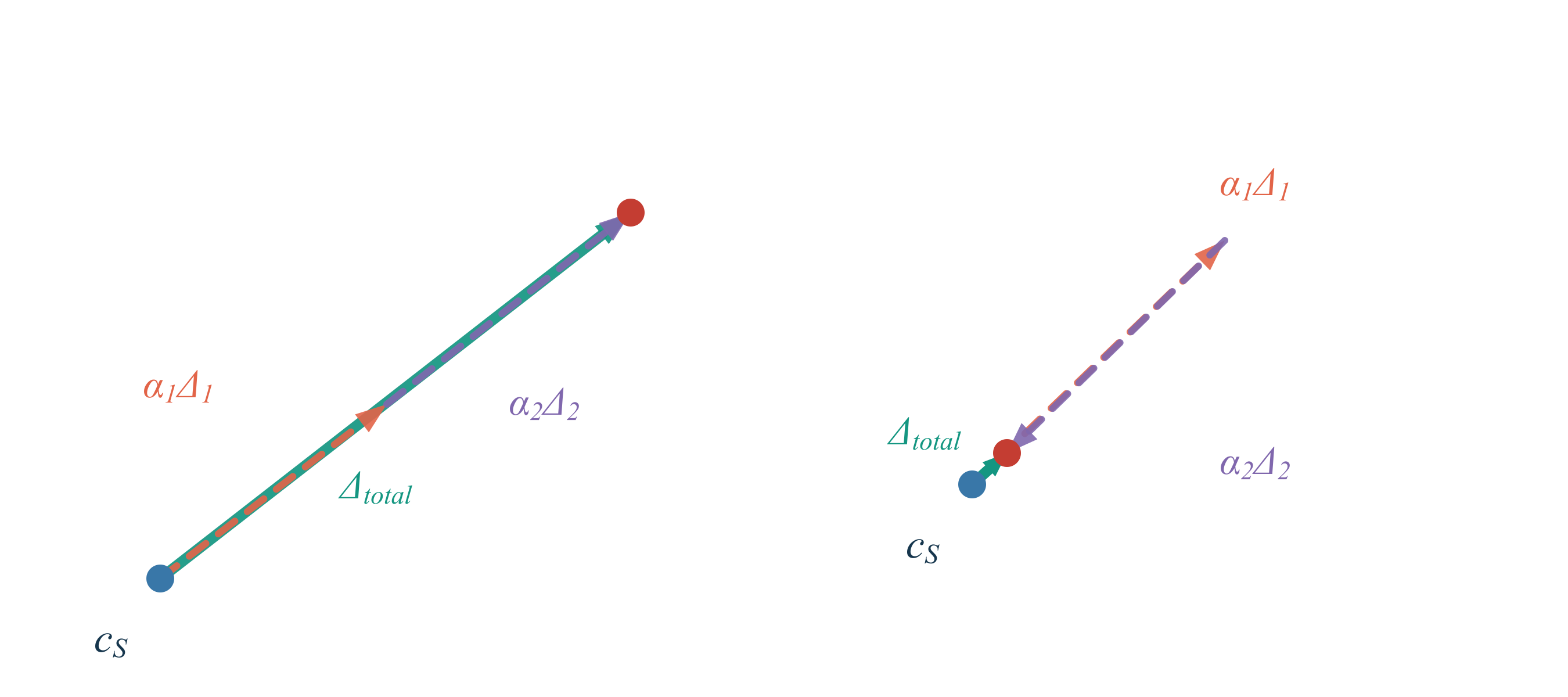

Although each teacher may be strong in isolation, together they may provide almost no effective target direction for the student.

The problem in multi-teacher distillation is not necessarily that the teachers are too weak. Their objectives may conflict with one another.

This conflict is often hard to see directly in probability space. In CLR space, it is simply a directional conflict between vectors.

We can quantify the consistency of two teachers directly with cosine similarity:

\[\operatorname{sim}(T_1,T_2) = \frac{ \Delta_1^\top\Delta_2 }{ \|\Delta_1\|_2 \|\Delta_2\|_2 }.\]

A value near $1$ means that the two teachers provide highly consistent distillation directions; a value near $0$ means that the directions are approximately orthogonal; and a value near $-1$ means that their learning signals are almost exactly opposed.

3.3. Monitoring Distillation Progress with CLR Vectors

CLR also gives us a natural way to observe how far distillation has progressed.

Suppose the target vector is $c_T$, and the student at training step $t$ is $c_S^{(t)}$.

Define the remaining distillation vector as

\[\Delta^{(t)} = c_T-c_S^{(t)}.\]

Then

\[\|\Delta^{(t)}\|_2\]

can be interpreted as the student’s remaining distance to the target in CLR space.

If distillation converges normally, we should observe

\[\|\Delta^{(t)}\|_2\rightarrow 0.\]

Distance alone, however, is not enough.

We can also examine the direction in which the student actually moves at each step:

\[u^{(t)} = c_S^{(t+1)}-c_S^{(t)}.\]

We then compare it with the target direction $\Delta^{(t)}$:

\[\cos\theta_t = \frac{ u^{(t)\top}\Delta^{(t)} }{ \|u^{(t)}\|_2 \|\Delta^{(t)}\|_2 }.\]

If $\cos\theta_t$ is close to $1$, the student is moving toward the target. If it is close to $0$, the update makes almost no progress toward the target. If it is negative, the student is moving away from the target.

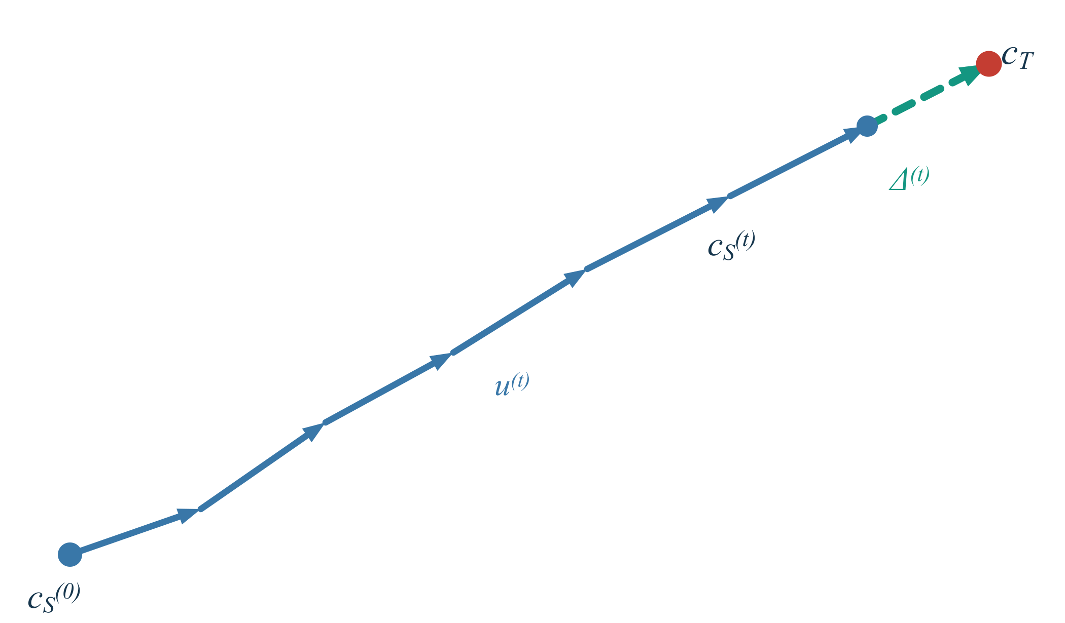
Instead of asking only

Is the loss decreasing?

we can ask directly

Is the student actually moving in the direction we intended?

In practice, $c_T$, $c_S^{(t)}$, and the corresponding metrics depend on the context. They should usually be averaged over a fixed set of prompts or evaluation contexts to produce comparable training curves.

4. Summary

This post develops a unified and intuitive perspective: distillation is not only about choosing a loss. More fundamentally, it is about specifying what we want the student to learn.

The CLR transformation maps a probability distribution into a zero-sum vector space while exactly preserving the log-ratios between classes. Differences between models can then be represented as directions, information from multiple teachers can be composed, and a particular capability can be extracted relative to a reference model.

From this perspective, distillation decomposes into three independent questions:

1. Where does the data come from? On-policy training uses trajectories or contexts visited by the student itself, whereas off-policy training uses data generated by another policy or drawn from a fixed dataset.
2. What is the target? In CLR space, we can copy a teacher or extract, scale, and combine information increments to construct the target distribution we actually want.
3. How do we approach the target? Once the target is fixed, we can choose Forward KL, Reverse KL, JSD, or another similarity measure.

This decomposition also gives us two direct analytical tools: the angles between teacher directions reveal supervision conflicts, while the student’s distance and direction of movement toward the target help us determine whether distillation is progressing as intended.

CLR does not decide what the best distillation target is. It does something more fundamental and useful: it makes the target hidden inside losses and probability distributions explicit, allowing us to construct the target we actually want before choosing how to match it.

Distill what you want: first decide what to distill, then decide how to distill it.

5. Citation

If you would like to cite this post in a paper, blog post, or other project, you can use the following format:

Zhang, Zhenyu. “Distill What You Want: A Unified View of On-Policy Distillation.” Zhenyu Zhang’s Blog (Aug. 2026). https://zhenyusteven.github.io/blog/distill-what-you-want/.

Or use BibTeX:

@article{zhang2026distill,
  title   = {Distill What You Want: A Unified View of On-Policy Distillation},
  author  = {Zhang, Zhenyu},
  journal = {zhenyusteven.github.io},
  year    = {2026},
  month   = {August},
  url     = "https://zhenyusteven.github.io/blog/distill-what-you-want/"
}

6. References

[1] Agarwal, Rishabh, Nino Vieillard, Yongchao Zhou, Piotr Stanczyk, Sabela Ramos, Matthieu Geist, and Olivier Bachem. “On-Policy Distillation of Language Models: Learning from Self-Generated Mistakes.” International Conference on Learning Representations (ICLR), 2024.

[2] Aitchison, John. “The Statistical Analysis of Compositional Data.” Journal of the Royal Statistical Society: Series B (Methodological), 44(2):139–160, 1982.

[3] Aitchison, John. The Statistical Analysis of Compositional Data. Chapman & Hall, 1986.

[4] Hinton, Geoffrey, Oriol Vinyals, and Jeff Dean. “Distilling the Knowledge in a Neural Network.” arXiv preprint arXiv:1503.02531, 2015.

[5] Feng, Shiyuan, Huan-ang Gao, Haohan Chi, Hanlin Wu, Zhilong Zhang, Zheng Jiang, Bingxiang He, Wei-Ying Ma, Ya-Qin Zhang, and Hao Zhou. “Weak-to-Strong Generalization via Direct On-Policy Distillation.” arXiv preprint arXiv:2607.05394, 2026.

[6] Xiaomi LLM-Core Team. “MiMo-V2-Flash Technical Report.” arXiv preprint arXiv:2601.02780, 2026.

[7] DeepSeek-AI. “DeepSeek-V4: Towards Highly Efficient Million-Token Context Intelligence.” arXiv preprint arXiv:2606.19348, 2026.

[8] Kullback, Solomon, and Richard A. Leibler. “On Information and Sufficiency.” The Annals of Mathematical Statistics, 22(1):79–86, 1951.

[9] Lin, Jianhua. “Divergence Measures Based on the Shannon Entropy.” IEEE Transactions on Information Theory, 37(1):145–151, 1991.